【原书作者】: Junichiro Toriwaki · Hiroyuki Yoshida
【页数 】:278
【开本 】 :16
【出版社】 :Springer
【出版日期】:May 2009
【文件格式】:pdf
【封面附图】:
【摘要或目录】:
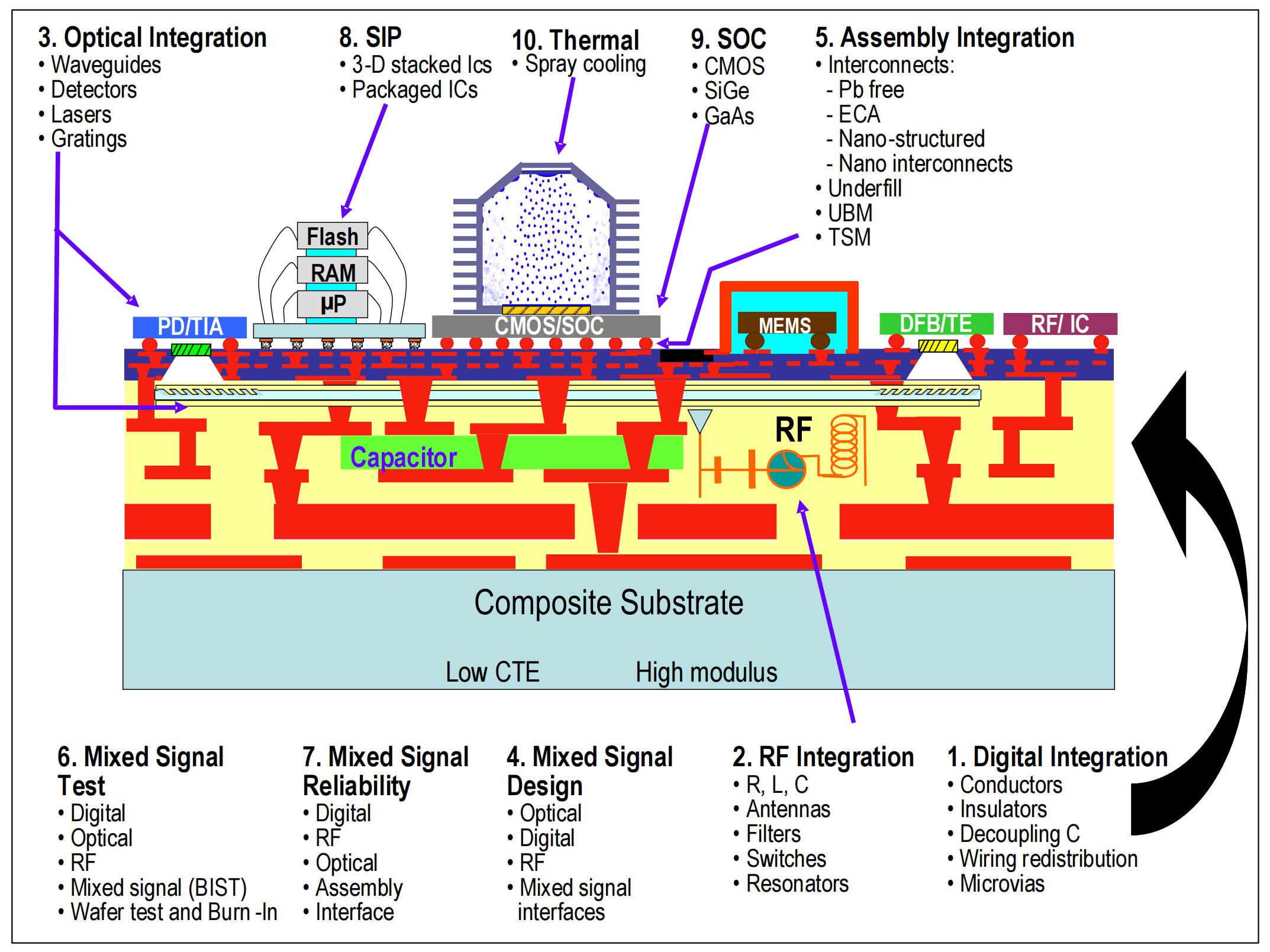
1 INTRODUCTION. . . . . . . . . . . . . . . . . . . . . . . . . . . . . . . . . . . . . . . . . 1
1.1 Overview . . . . . . . . . . . . . . . . . . . . . . . . . . . . . . . . . . . . . . . . . . . . . . . 1
1.1.1 3D continuous images . . . . . . . . . . . . . . . . . . . . . . . . . . . . . . 1
1.1.2 3D digital images. . . . . . . . . . . . . . . . . . . . . . . . . . . . . . . . . . 1
1.2 What does “3D image” mean? . . . . . . . . . . . . . . . . . . . . . . . . . . . . 3
1.2.1 Dimensionality of the media and of the subject . . . . . . . . 3
1.2.2 Types of 3D images. . . . . . . . . . . . . . . . . . . . . . . . . . . . . . . . 3
1.2.3 Cues for 3D information. . . . . . . . . . . . . . . . . . . . . . . . . . . . 5
1.2.4 Specific examples of 3D images . . . . . . . . . . . . . . . . . . . . . . 5
1.3 Types and characteristics of 3D image processing . . . . . . . . . . . . 12
1.3.1 Examples of 3D image processing. . . . . . . . . . . . . . . . . . . . 12
1.3.2 Virtual spaces as 3D digital images . . . . . . . . . . . . . . . . . . 13
1.3.3 Characteristics of 3D image processing . . . . . . . . . . . . . . . 14
1.3.4 Objectives in 3D image processing . . . . . . . . . . . . . . . . . . . 15
1.4 The contents of this book. . . . . . . . . . . . . . . . . . . . . . . . . . . . . . . . . 18
2 MODELS OF IMAGES AND IMAGE OPERATIONS. . . . . 21
2.1 Introduction . . . . . . . . . . . . . . . . . . . . . . . . . . . . . . . . . . . . . . . . . . . . 21
2.2 Continuous and digitized images. . . . . . . . . . . . . . . . . . . . . . . . . . . 22
2.2.1 Continuous images . . . . . . . . . . . . . . . . . . . . . . . . . . . . . . . . 22
2.2.2 Digitized images . . . . . . . . . . . . . . . . . . . . . . . . . . . . . . . . . . 22
2.2.3 Three-dimensional images . . . . . . . . . . . . . . . . . . . . . . . . . . 24
2.2.4 3D line figures and digitization . . . . . . . . . . . . . . . . . . . . . . 26
2.2.5 Cross section and projection . . . . . . . . . . . . . . . . . . . . . . . . 29
2.2.6 Relationships among images . . . . . . . . . . . . . . . . . . . . . . . . 31
2.3 Model of image operations . . . . . . . . . . . . . . . . . . . . . . . . . . . . . . . . 32
2.3.1 Formulation of image operations . . . . . . . . . . . . . . . . . . . . 33
2.3.2 Relations between image operators . . . . . . . . . . . . . . . . . . 34
2.3.3 Binary operators between images . . . . . . . . . . . . . . . . . . . . 34
2.3.4 Composition of image operations . . . . . . . . . . . . . . . . . . . . 35
2.3.5 Basic operators . . . . . . . . . . . . . . . . . . . . . . . . . . . . . . . . . . . 38
XII Contents
2.4 Algorithm of image operations . . . . . . . . . . . . . . . . . . . . . . . . . . . . 40
2.4.1 General form of image operations. . . . . . . . . . . . . . . . . . . . 41
2.4.2 Important types of algorithms . . . . . . . . . . . . . . . . . . . . . . 41
3 LOCAL PROCESSING OF 3D IMAGES . . . . . . . . . . . . . . . . . . 49
3.1 Classification of local operations . . . . . . . . . . . . . . . . . . . . . . . . . . . 49
3.1.1 General form . . . . . . . . . . . . . . . . . . . . . . . . . . . . . . . . . . . . . 49
3.1.2 Classification by functions of filters . . . . . . . . . . . . . . . . . . 50
3.1.3 Classification by the form of a local function . . . . . . . . . . 50
3.2 Smoothing filter . . . . . . . . . . . . . . . . . . . . . . . . . . . . . . . . . . . . . . . . . 51
3.2.1 Linear smoothing filter . . . . . . . . . . . . . . . . . . . . . . . . . . . . . 51
3.2.2 Median filter and order statistics filter . . . . . . . . . . . . . . . 52
3.2.3 Edge-preserving smoothing . . . . . . . . . . . . . . . . . . . . . . . . . 53
3.2.4 Morphology filter . . . . . . . . . . . . . . . . . . . . . . . . . . . . . . . . . . 54
3.3 Difference filter. . . . . . . . . . . . . . . . . . . . . . . . . . . . . . . . . . . . . . . . . . 56
3.3.1 Significance . . . . . . . . . . . . . . . . . . . . . . . . . . . . . . . . . . . . . . . 56
3.3.2 Differentials in continuous space . . . . . . . . . . . . . . . . . . . . . 57
3.3.3 Derivatives in digitized space . . . . . . . . . . . . . . . . . . . . . . . 58
3.3.4 Basic characteristics of difference filter . . . . . . . . . . . . . . . 59
3.3.5 Omnidirectionalization . . . . . . . . . . . . . . . . . . . . . . . . . . . . . 60
3.3.6 1D difference filters and their combinations . . . . . . . . . . . 61
3.3.7 3D Laplacian . . . . . . . . . . . . . . . . . . . . . . . . . . . . . . . . . . . . . 62
3.3.8 2D difference filters and their combination . . . . . . . . . . . . 62
3.4 Differential features of a curved surface. . . . . . . . . . . . . . . . . . . . . 66
3.5 Region growing (region merging) . . . . . . . . . . . . . . . . . . . . . . . . . . 69
3.5.1 Outline . . . . . . . . . . . . . . . . . . . . . . . . . . . . . . . . . . . . . . . . . . 69
3.5.2 Region expansion. . . . . . . . . . . . . . . . . . . . . . . . . . . . . . . . . . 69
4 GEOMETRICAL PROPERTIES OF 3D DIGITIZED
IMAGES . . . . . . . . . . . . . . . . . . . . . . . . . . . . . . . . . . . . . . . . . . . . . . . . . . 73
4.1 Neighborhood and connectivity. . . . . . . . . . . . . . . . . . . . . . . . . . . . 73
4.1.1 Neighborhood. . . . . . . . . . . . . . . . . . . . . . . . . . . . . . . . . . . . . 73
4.1.2 Connectivity and connected component . . . . . . . . . . . . . . 75
4.2 Simplex and simplicial decomposition . . . . . . . . . . . . . . . . . . . . . . 78
4.3 Euler number . . . . . . . . . . . . . . . . . . . . . . . . . . . . . . . . . . . . . . . . . . . 80
4.4 Local feature of a connected component and topology of a
figure . . . . . . . . . . . . . . . . . . . . . . . . . . . . . . . . . . . . . . . . . . . . . . . . . . 81
4.5 Local patterns and their characterization . . . . . . . . . . . . . . . . . . . 85
4.5.1 2 × 2 × 2 local patterns. . . . . . . . . . . . . . . . . . . . . . . . . . . . 86
4.5.2 3 × 3 × 3 local patterns. . . . . . . . . . . . . . . . . . . . . . . . . . . . 87
4.5.3 Classification of the voxel state. . . . . . . . . . . . . . . . . . . . . . 89
4.5.4 Voxel state and connectivity index . . . . . . . . . . . . . . . . . . . 90
4.6 Calculation of connectivity index and connectivity number . . . . 92
4.6.1 Basic ideas . . . . . . . . . . . . . . . . . . . . . . . . . . . . . . . . . . . . . . . 92
4.6.2 Calculation of the connectivity index. . . . . . . . . . . . . . . . . 92
Contents XIII
4.6.3 Calculation of the connectivity number . . . . . . . . . . . . . . . 93
4.7 Calculation of the Euler number . . . . . . . . . . . . . . . . . . . . . . . . . . . 94
4.7.1 Triangulation method . . . . . . . . . . . . . . . . . . . . . . . . . . . . . . 95
4.7.2 Simplex counting method. . . . . . . . . . . . . . . . . . . . . . . . . . . 97
4.8 Algorithm of deletability test . . . . . . . . . . . . . . . . . . . . . . . . . . . . . 101
4.9 Path and distance functions. . . . . . . . . . . . . . . . . . . . . . . . . . . . . . . 103
4.9.1 Path . . . . . . . . . . . . . . . . . . . . . . . . . . . . . . . . . . . . . . . . . . . . . 103
4.9.2 Distance function. . . . . . . . . . . . . . . . . . . . . . . . . . . . . . . . . . 105
4.9.3 Distance function in applications . . . . . . . . . . . . . . . . . . . . 109
4.9.4 Improvement in distance metric . . . . . . . . . . . . . . . . . . . . . 110
4.10 Border surface . . . . . . . . . . . . . . . . . . . . . . . . . . . . . . . . . . . . . . . . . . 113
5 ALGORITHM OF BINARY IMAGE PROCESSING . . . . . . 115
5.1 Introduction . . . . . . . . . . . . . . . . . . . . . . . . . . . . . . . . . . . . . . . . . . . . 115
5.2 Labeling of a connected component . . . . . . . . . . . . . . . . . . . . . . . . 116
5.3 Shrinking. . . . . . . . . . . . . . . . . . . . . . . . . . . . . . . . . . . . . . . . . . . . . . . 117
5.4 Surface thinning and axis thinning . . . . . . . . . . . . . . . . . . . . . . . . . 120
5.4.1 Definition . . . . . . . . . . . . . . . . . . . . . . . . . . . . . . . . . . . . . . . . 120
5.4.2 Requirements of thinning . . . . . . . . . . . . . . . . . . . . . . . . . . . 122
5.4.3 Realization - the sequential type . . . . . . . . . . . . . . . . . . . . 122
5.4.4 Examples of surface/axis thinning algorithms
(sequential type) . . . . . . . . . . . . . . . . . . . . . . . . . . . . . . . . . . 124
5.4.5 Surface thinning algorithm accompanying the
Euclidean distance transformation . . . . . . . . . . . . . . . . . . . 127
5.4.6 Use of a 1D list for auxiliary information . . . . . . . . . . . . . 131
5.4.7 Examples of surface/axis thinning algorithm (parallel
type) . . . . . . . . . . . . . . . . . . . . . . . . . . . . . . . . . . . . . . . . . . . . 136
5.4.8 Experimental results . . . . . . . . . . . . . . . . . . . . . . . . . . . . . . . 137
5.4.9 Points in algorithm construction. . . . . . . . . . . . . . . . . . . . . 138
5.5 Distance transformation and skeleton . . . . . . . . . . . . . . . . . . . . . . 144
5.5.1 Definition . . . . . . . . . . . . . . . . . . . . . . . . . . . . . . . . . . . . . . . . 144
5.5.2 Significance of DT and skeleton . . . . . . . . . . . . . . . . . . . . . 146
5.5.3 Classification of algorithms . . . . . . . . . . . . . . . . . . . . . . . . . 147
5.5.4 Example of an algorithm – (1) squared Euclidean DT . . 147
5.5.5 Example of algorithms – (2) variable neighborhood
DT (parallel type) . . . . . . . . . . . . . . . . . . . . . . . . . . . . . . . . . 153
5.5.6 Supplementary comments on algorithms of DT . . . . . . . . 156
5.5.7 Skeleton. . . . . . . . . . . . . . . . . . . . . . . . . . . . . . . . . . . . . . . . . . 158
5.5.8 Reverse distance transformation . . . . . . . . . . . . . . . . . . . . . 161
5.5.9 Example of RDT algorithms – (1) Euclidean squared
RDT . . . . . . . . . . . . . . . . . . . . . . . . . . . . . . . . . . . . . . . . . . . . 162
5.5.10 Example of RDT algorithm – (2) fixed neighborhood
(6-, 18-, or 26-neighborhood) RDT (sequential type) . . . 167
5.5.11 Extraction of skeleton. . . . . . . . . . . . . . . . . . . . . . . . . . . . . . 170
5.5.12 Distance transformation of a line figure . . . . . . . . . . . . . . 176
XIV Contents
5.6 Border surface following . . . . . . . . . . . . . . . . . . . . . . . . . . . . . . . . . . 176
5.6.1 Outline . . . . . . . . . . . . . . . . . . . . . . . . . . . . . . . . . . . . . . . . . . 176
5.6.2 Examples of algorithm . . . . . . . . . . . . . . . . . . . . . . . . . . . . . 179
5.6.3 Restoration of a figure . . . . . . . . . . . . . . . . . . . . . . . . . . . . . 181
5.7 Knot and link . . . . . . . . . . . . . . . . . . . . . . . . . . . . . . . . . . . . . . . . . . . 182
5.7.1 Outline . . . . . . . . . . . . . . . . . . . . . . . . . . . . . . . . . . . . . . . . . . 182
5.7.2 Reduction of a digital knot . . . . . . . . . . . . . . . . . . . . . . . . . 184
5.8 Voronoi division of a digitized image . . . . . . . . . . . . . . . . . . . . . . . 186
6 ALGORITHMS FOR PROCESSING CONNECTED
COMPONENTS WITH GRAY VALUES . . . . . . . . . . . . . . . . . . 191
6.1 Distance transformation of a gray-tone image . . . . . . . . . . . . . . . 191
6.1.1 Definition . . . . . . . . . . . . . . . . . . . . . . . . . . . . . . . . . . . . . . . . 191
6.1.2 An example of algorithm . . . . . . . . . . . . . . . . . . . . . . . . . . . 192
6.2 Thinning of a gray-tone image . . . . . . . . . . . . . . . . . . . . . . . . . . . . 194
6.2.1 Basic idea . . . . . . . . . . . . . . . . . . . . . . . . . . . . . . . . . . . . . . . . 194
6.2.2 Requirements . . . . . . . . . . . . . . . . . . . . . . . . . . . . . . . . . . . . . 195
6.2.3 Principles of thinning . . . . . . . . . . . . . . . . . . . . . . . . . . . . . . 195
6.3 Examples of algorithms – (1) integration of information
concerning density values . . . . . . . . . . . . . . . . . . . . . . . . . . . . . . . . . 197
6.3.1 Algorithm . . . . . . . . . . . . . . . . . . . . . . . . . . . . . . . . . . . . . . . . 197
6.3.2 Experimental results . . . . . . . . . . . . . . . . . . . . . . . . . . . . . . . 200
6.4 Examples of algorithms – (2) ridgeline following . . . . . . . . . . . . . 203
6.4.1 Meanings of a ridgeline. . . . . . . . . . . . . . . . . . . . . . . . . . . . . 203
6.4.2 Algorithm . . . . . . . . . . . . . . . . . . . . . . . . . . . . . . . . . . . . . . . . 204
6.4.3 Experiments . . . . . . . . . . . . . . . . . . . . . . . . . . . . . . . . . . . . . . 207
7 VISUALIZATION OF 3D GRAY-TONE IMAGES . . . . . . . . 209
7.1 Formulation of visualization problem. . . . . . . . . . . . . . . . . . . . . . . 209
7.2 Voxel data and the polygon model . . . . . . . . . . . . . . . . . . . . . . . . . 211
7.2.1 Voxel surface representation . . . . . . . . . . . . . . . . . . . . . . . . 211
7.2.2 Marching cubes algorithm . . . . . . . . . . . . . . . . . . . . . . . . . . 211
7.3 Cross section, surface, and projection . . . . . . . . . . . . . . . . . . . . . . 214
7.3.1 Cross section . . . . . . . . . . . . . . . . . . . . . . . . . . . . . . . . . . . . . 214
7.3.2 Surface. . . . . . . . . . . . . . . . . . . . . . . . . . . . . . . . . . . . . . . . . . . 215
7.3.3 Projection . . . . . . . . . . . . . . . . . . . . . . . . . . . . . . . . . . . . . . . . 216
7.4 The concept of visualization based on ray casting – (1)
projection of a point . . . . . . . . . . . . . . . . . . . . . . . . . . . . . . . . . . . . . 218
7.4.1 Displaying a point . . . . . . . . . . . . . . . . . . . . . . . . . . . . . . . . . 218
7.4.2 Displaying lines . . . . . . . . . . . . . . . . . . . . . . . . . . . . . . . . . . . 221
7.4.3 Displaying surfaces . . . . . . . . . . . . . . . . . . . . . . . . . . . . . . . . 221
7.5 The concept of visualization based on ray casting – (2)
manipulation of density values . . . . . . . . . . . . . . . . . . . . . . . . . . . . 222
7.6 Rendering surfaces based on ray casting – surface rendering . . . 222
7.6.1 Calculation of the brightness of a surface . . . . . . . . . . . . . 223
Contents XV
7.6.2 Smooth shading . . . . . . . . . . . . . . . . . . . . . . . . . . . . . . . . . . . 225
7.6.3 Depth coding . . . . . . . . . . . . . . . . . . . . . . . . . . . . . . . . . . . . . 227
7.6.4 Ray tracing . . . . . . . . . . . . . . . . . . . . . . . . . . . . . . . . . . . . . . . 227
7.7 Photorealistic rendering and rendering for visualization . . . . . . . 230
7.8 Displaying density values based on ray casting – volume
rendering . . . . . . . . . . . . . . . . . . . . . . . . . . . . . . . . . . . . . . . . . . . . . . . 231
7.8.1 The algorithm of volume rendering . . . . . . . . . . . . . . . . . . 231
7.8.2 Selection of parameters . . . . . . . . . . . . . . . . . . . . . . . . . . . . 233
7.8.3 Front-to-back algorithm . . . . . . . . . . . . . . . . . . . . . . . . . . . . 235
7.8.4 Properties of volume rendering and surface rendering . . 236
7.8.5 Gradient shading . . . . . . . . . . . . . . . . . . . . . . . . . . . . . . . . . . 240
References . . . . . . . . . . . . . . . . . . . . . . . . . . . . . . . . . . . . . . . . . . . . . . . . . . . . . 243
 求助 Fundamentals of Three-Dimensional Digital Image Processing: Fundamentals of Three-Dimensional DIP.part1.rar